Fit a curved line

This notebook will help you plot the strength-duration curve for your earthworm.

Note: If you’re new to Jupyter Notebooks and/or Python, please be sure to work through the Introduction notebook before this one.

Step 1. Define values to plot

With matplotlib imported, we can now use the scatter function by calling plt.scatter(). However, we need to define what to plot first. One straightforward way to think about this is to define an x variable and a y variable. Below, there are lists of values (defined in brackets [ ]) assigned to x and y. Replace these with your own values, depending on what you’d like to plot on the x and y axis of your strength duration curve.

Note: Remember that in a scatterplot, each dot has both an x and a y value. Therefore, these lists should be the same length. The coordinate for each point will be the values at the same index in x and y. For example, the coordinate for the very first point will be x[0],y[0].

# Add your data points here
x = [1,2,3,4,5,6]
y = [1,0.8,0.5,0.45,0.4,0.4]

%whos

Variable   Type    Data/Info
----------------------------
x          list    n=6
y          list    n=6

Step 2. Fit a hyperbolic curve to hypothetical data

The strength-duration curve should follow a hyperbolic function:

\[ a = r + \frac{r*c}{t} \]

where a is the stimulus amplitude (in amps or volts), r is the rheobase, c is the chronaxie, and t is time (the width of the stimulus).

We’ll first define that function below:

# Define the hyperbolic curve function
def func(t, r, c):
    return r+((r*c)/t) #hyperbolic function

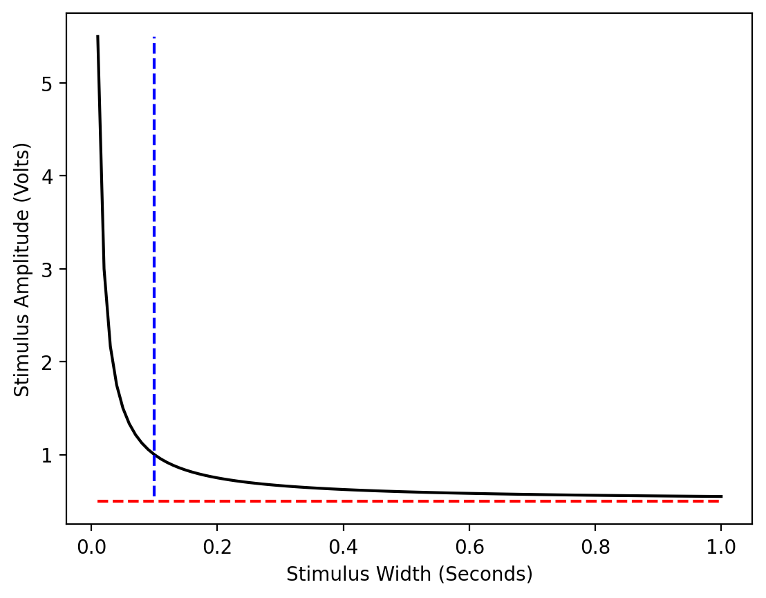
To demonstrate what this function looks like, we’ll use np.linspace() to generate a list of 100 numbers from 0 to 1, with 0.01 spacing. We’ll also define a sample rheobase and chronaxie. Then, from those points, we’ll fit a hyperbolic curve using scipy.optimize.curve_fit(), which uses non-linear least squares to fit a function to data. See the curve_fit documentation.

# Import numpy & curve fitting package
import numpy as np
from scipy.optimize import curve_fit

# Import & configure plotting packages
import matplotlib.pyplot as plt
%matplotlib inline 
%config InlineBackend.figure_format = 'retina'

# Define pulse
pulse_width = np.linspace(0.01,1,100)
rheobase = .5 # in V
chronaxie = 0.1 # in ms

amplitude = rheobase+((rheobase*chronaxie)/pulse_width)

# Use our function & fit the curve!
sample_popt, sample_pcov = curve_fit(func,pulse_width,amplitude)

# Plot a regression line, using the slope & intercept
plt.plot(pulse_width, func(pulse_width, *sample_popt), 'black')

# Plot chronaxie & rheobase lines
plt.vlines(chronaxie,amplitude.min(),amplitude.max(),color='blue',linestyle='--')
plt.hlines(rheobase,pulse_width.min(),pulse_width.max(),color='red',linestyle='--')

# Label the axes & show plot
plt.ylabel('Stimulus Amplitude (Volts)')
plt.xlabel('Stimulus Width (Seconds)')

plt.show()

/Users/ashley/anaconda3/envs/jb/lib/python3.11/site-packages/IPython/core/pylabtools.py:152: MatplotlibDeprecationWarning: savefig() got unexpected keyword argument "orientation" which is no longer supported as of 3.3 and will become an error two minor releases later
  fig.canvas.print_figure(bytes_io, **kw)
/Users/ashley/anaconda3/envs/jb/lib/python3.11/site-packages/IPython/core/pylabtools.py:152: MatplotlibDeprecationWarning: savefig() got unexpected keyword argument "facecolor" which is no longer supported as of 3.3 and will become an error two minor releases later
  fig.canvas.print_figure(bytes_io, **kw)
/Users/ashley/anaconda3/envs/jb/lib/python3.11/site-packages/IPython/core/pylabtools.py:152: MatplotlibDeprecationWarning: savefig() got unexpected keyword argument "edgecolor" which is no longer supported as of 3.3 and will become an error two minor releases later
  fig.canvas.print_figure(bytes_io, **kw)
/Users/ashley/anaconda3/envs/jb/lib/python3.11/site-packages/IPython/core/pylabtools.py:152: MatplotlibDeprecationWarning: savefig() got unexpected keyword argument "bbox_inches_restore" which is no longer supported as of 3.3 and will become an error two minor releases later
  fig.canvas.print_figure(bytes_io, **kw)

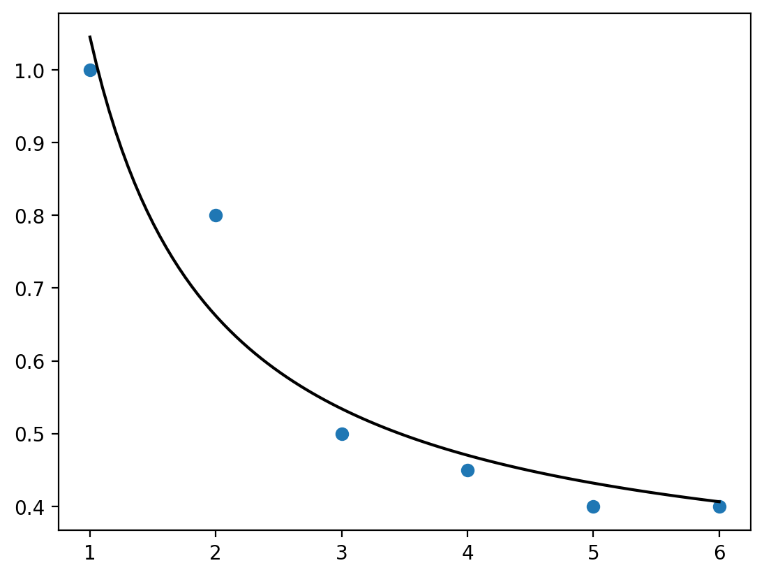
Step 3. Fit a hyperbolic curve to your data

Above, you can see a perfectly fit curve, with the rheobase and chronaxie labeled.

Now, let’s do the same, but with your data.

# Transform x & y data into arrays
x = np.array(x)
y = np.array(y)

# Fit the curve with your data!
popt, pcov = curve_fit(func,x,y)

# Generate additional x-values to make a smoooth curve
xnew = np.linspace(x.min(),x.max(), 100)

# Plot a regression line, using the slope & intercept
plt.plot(xnew, func(xnew, *popt), 'black')
plt.scatter(x,y)

# Optional -- can you figure out how to add rheobase & chronaxie?

# Add your labels here!

plt.show()

/Users/ashley/anaconda3/envs/jb/lib/python3.11/site-packages/IPython/core/pylabtools.py:152: MatplotlibDeprecationWarning: savefig() got unexpected keyword argument "orientation" which is no longer supported as of 3.3 and will become an error two minor releases later
  fig.canvas.print_figure(bytes_io, **kw)

/Users/ashley/anaconda3/envs/jb/lib/python3.11/site-packages/IPython/core/pylabtools.py:152: MatplotlibDeprecationWarning: savefig() got unexpected keyword argument "facecolor" which is no longer supported as of 3.3 and will become an error two minor releases later
  fig.canvas.print_figure(bytes_io, **kw)
/Users/ashley/anaconda3/envs/jb/lib/python3.11/site-packages/IPython/core/pylabtools.py:152: MatplotlibDeprecationWarning: savefig() got unexpected keyword argument "edgecolor" which is no longer supported as of 3.3 and will become an error two minor releases later
  fig.canvas.print_figure(bytes_io, **kw)
/Users/ashley/anaconda3/envs/jb/lib/python3.11/site-packages/IPython/core/pylabtools.py:152: MatplotlibDeprecationWarning: savefig() got unexpected keyword argument "bbox_inches_restore" which is no longer supported as of 3.3 and will become an error two minor releases later
  fig.canvas.print_figure(bytes_io, **kw)

It is also important to know how well our curve fits. To do so, we’ll calculate the residuals and then the sum of squares.

#  Calculate the distance (on y axis) from data to curve
residuals = y - func(x, *popt)

# Calculate the residual sum of squares
ss_res = np.sum(residuals**2)

# Calculate the total sum of squares
ss_tot = np.sum((y-np.mean(y))**2)

# Calculate r-squared
r_squared = 1 - (ss_res / ss_tot)

print('R^2 = ',r_squared)
print('Rheobase: ' , popt[0])
print('Chronaxie:  ', popt[1])

R^2 =  0.9239011751642454
Rheobase:  0.278745874411597
Chronaxie:   2.749230408204977